Chapter 1. Reliable, Scalable, and Maintainable Applications

Thinking About Data Systems

Increasingly many applications now have such demanding or wide-ranging requirements that a single tool can no longer meet all of its data processing and storage needs. Instead, the work is broken down into tasks that can be performed efficiently on a single tool, and those different tools are stitched together using application code.（在应用层代码整合多种不同的工具来实现需求）

In this book, we focus on three concerns that are important in most software systems:

Reliability

The system should continue to work correctly (performing the correct function at the desired level of performance) even in the face of adversity (hardware or software faults, and even human error)
Scalability

As the system grows (in data volume, traffic volume, or complexity), there should be reasonable ways of dealing with that growth
Maintainability

Over time, many different people will work on the system (engineering and operations, both maintaining current behavior and adapting the system to new use cases), and they should all be able to work on it productively.

Reliability

Continuing to work correctly, even when things go wrong. A fault is not the same as a failure. A fault is usually defined as one component of the system deviating from its spec, whereas a failure is when the system as a whole stops providing the required service to the user. It is impossible to reduce the probability of a fault to zero; therefore it is usually best to design fault-tolerance mechanisms that prevent faults from causing failures.（实现 fault－tolerance 以避免 faults 引发 failures）

Scalability

Scalability is the term we use to describe a system’s ability to cope with increased load.

Describing Load

Load can be described with a few numbers which we call load parameters. The best choice of parameters depends on the architecture of your system: it may be requests per second to a web server, the ratio of reads to writes in a database, the number of simultaneously active users in a chat room, the hit rate on a cache, or something else.

Approaches for Coping with Load

People often talk of a dichotomy between scaling up (vertical scaling, moving to a more powerful machine) and scaling out (horizontal scaling, distributing the load across multiple smaller machines). Distributing load across multiple machines is also known as a shared-nothing architecture.

An architecture that scales well for a particular application is built around assumptions of which operations will be common and which will be rare—the load parameters（扩展性良好的系统是基于 load parameter 来构建的）.

Maintainability

Operability: Making Life Easy for Operations

Make it easy for operations teams to keep the system running smoothly.

Simplicity:Managing Complexity

Make it easy for new engineers to understand the system, by removing as much complexity as possible from the system. (Note this is not the same as simplicity of the user interface.) One of the best tools we have for removing accidental complexity is abstraction. A good abstraction can hide a great deal of implementation detail behind a clean, simple-to-understand façade. SQL is an abstraction that hides complex on-disk and in-memory data structures.

Evolvability: Making Change Easy

Make it easy for engineers to make changes to the system in the future, adapting it for unanticipated use cases as requirements change. Also known as extensibility, modifiability, or plasticity.

Chapter 2. Data Models and Query Languages

Data models are perhaps the most important part of developing software, because they have such a profound effect: not only on how the software is written, but also on how we think about the problem that we are solving.

Most applications are built by layering one data model on top of another. For each layer, the key question is: how is it represented in terms of the next-lower layer? In a complex application there may be more intermediary levels, such as APIs built upon APIs, but the basic idea is still the same: each layer hides the complexity of the layers below it by providing a clean data model.

Relational Model Versus Document Model

The best-known data model today is probably that of SQL, data is organized into relations (called tables in SQL), where each relation is an unordered collection of tuples (rows in SQL).

The Birth of NoSQL

There are several driving forces behind the adoption of NoSQL databases, including:

A need for greater scalability than relational databases can easily achieve, including very large datasets or very high write throughput
A widespread preference for free and open source software over commercial database products
Specialized query operations that are not well supported by the relational model
Frustration with the restrictiveness of relational schemas, and a desire for a more dynamic and expressive data model

Relational Versus Document Databases Today

The main arguments in favor of the document data model are schema flexibility, better performance due to locality, and that for some applications it is closer to the data structures used by the application.（不需要和关系型数据库一样使用 ORM 做转换：If data is stored in relational tables, an awkward translation layer is required between the objects in the application code and the database model of tables, rows, and columns. The disconnect between the models is sometimes called an impedance mismatch）The relational model counters by providing better support for joins, and many-to-one and many-to-many relationships.

Which data model leads to simpler application code?

If the data in your application has a document-like structure, then it’s probably a good idea to use a document model. However, if your application does use many-to-many relationships, the document model becomes less appealing. It’s possible to reduce the need for joins by denormalizing, but then the application code needs to do additional work to keep the denormalized data consistent. Joins can be emulated in application code by making multiple requests to the database, but that also moves complexity into the application and is usually slower than a join performed by specialized code inside the database. In such cases, using a document model can lead to significantly more complex application code and worse performance.

Schema flexibility in the document model

Document databases are sometimes called schemaless, there is an implicit schema, but it is not enforced by the database. A more accurate term is schema-on-read (the structure of the data is implicit, and only interpreted when the data is read), in contrast with schema-on-write (the traditional approach of relational databases, where the schema is explicit and the database ensures all written data conforms to it).

Data locality for queries

A document is usually stored as a single continuous string, encoded as JSON, XML, or a binary variant thereof. If your application often needs to access the entire document, there is a performance advantage to this storage locality.

The locality advantage only applies if you need large parts of the document at the same time. On updates to a document, the entire document usually needs to be rewritten—only modifications that don’t change the encoded size of a document can easily be performed in place. For these reasons, it is generally recommended that you keep documents fairly small and avoid writes that increase the size of a document.

Query Languages for Data

When the relational model was introduced, it included a new way of querying data: SQL is a declarative query language, whereas IMS and CODASYL queried the database using imperative code.

In a declarative query language, like SQL or relational algebra, you just specify the pattern of the data you want, but not how to achieve that goal.

Declarative languages often lend themselves to parallel execution. Imperative code is very hard to parallelize across multiple cores and multiple machines, because it specifies instructions that must be performed in a particular order.

Graph-Like Data Models

The relational model can handle simple cases of many-to-many relationships, but as the connections within your data become more complex, it becomes more natural to start modeling your data as a graph.

Property Graphs

In the property graph model, each vertex consists of:

A unique identifier
A set of outgoing edges
A set of incoming edges
A collection of properties (key-value pairs)

Each edge consists of:

A unique identifier
The vertex at which the edge starts (the tail vertex)
The vertex at which the edge ends (the head vertex)
A label to describe the kind of relationship between the two vertices
A collection of properties (key-value pairs)

Graphs are good for evolvability: as you add features to your application, a graph can easily be extended to accommodate changes in your application’s data structures.

Chapter 3. Storage and Retrieval

We will examine two families of storage engines: log-structured storage engines, and page-oriented storage engines such as B-trees.

Data Structures That Power Your Database

In order to efficiently find the value for a particular key in the database, we need a different data structure: an index.

Hash Indexes

Let’s say our data storage consists only of appending to a file. Then the simplest possible indexing strategy is this: keep an in-memory hash map where every key is mapped to a byte offset in the data file—the location at which the value can be found. This is essentially what Bitcask (the default storage engine in Riak) does.

A storage engine like Bitcask is well suited to situations where the value for each key is updated frequently. For example, the key might be the URL of a cat video, and the value might be the number of times it has been played. In this kind of workload, there are a lot of writes, but there are not too many distinct keys—you have a large number of writes per key, but it’s feasible to keep all keys in memory.

How do we avoid eventually running out of disk space? A good solution is to break the log into segments of a certain size by closing a segment file when it reaches a certain size, and making subsequent writes to a new segment file. We can then perform compaction on these segments. Compaction means throwing away duplicate keys in the log, and keeping only the most recent update for each key.

Each segment now has its own in-memory hash table, mapping keys to file offsets. In order to find the value for a key, we first check the most recent segment’s hash map; if the key is not present we check the second-most-recent segment, and so on.

An append-only design turns out to be good for several reasons:

Appending and segment merging are sequential write operations, which are generally much faster than random writes, especially on magnetic spinning-disk hard drives.
Concurrency and crash recovery are much simpler if segment files are append-only or immutable.
Merging old segments avoids the problem of data files getting fragmented over time.

However, the hash table index also has limitations:

The hash table must fit in memory, so if you have a very large number of keys, you’re out of luck.
Range queries are not efficient.

SSTables and LSM-Trees

Now we can make a simple change to the format of our segment files: we require that the sequence of key-value pairs is sorted by key.

We call this format Sorted String Table, or SSTable for short. We also require that each key only appears once within each merged segment file (the compaction process already ensures that). SSTables have several big advantages over log segments with hash indexes:

Merging segments is simple and efficient, even if the files are bigger than the available memory. The approach is like the one used in the mergesort algorithm.
In order to find a particular key in the file, you no longer need to keep an index of all the keys in memory. You still need an in-memory index to tell you the offsets for some of the keys, but it can be sparse: one key for every few kilobytes of segment file is sufficient, because a few kilobytes can be scanned very quickly.

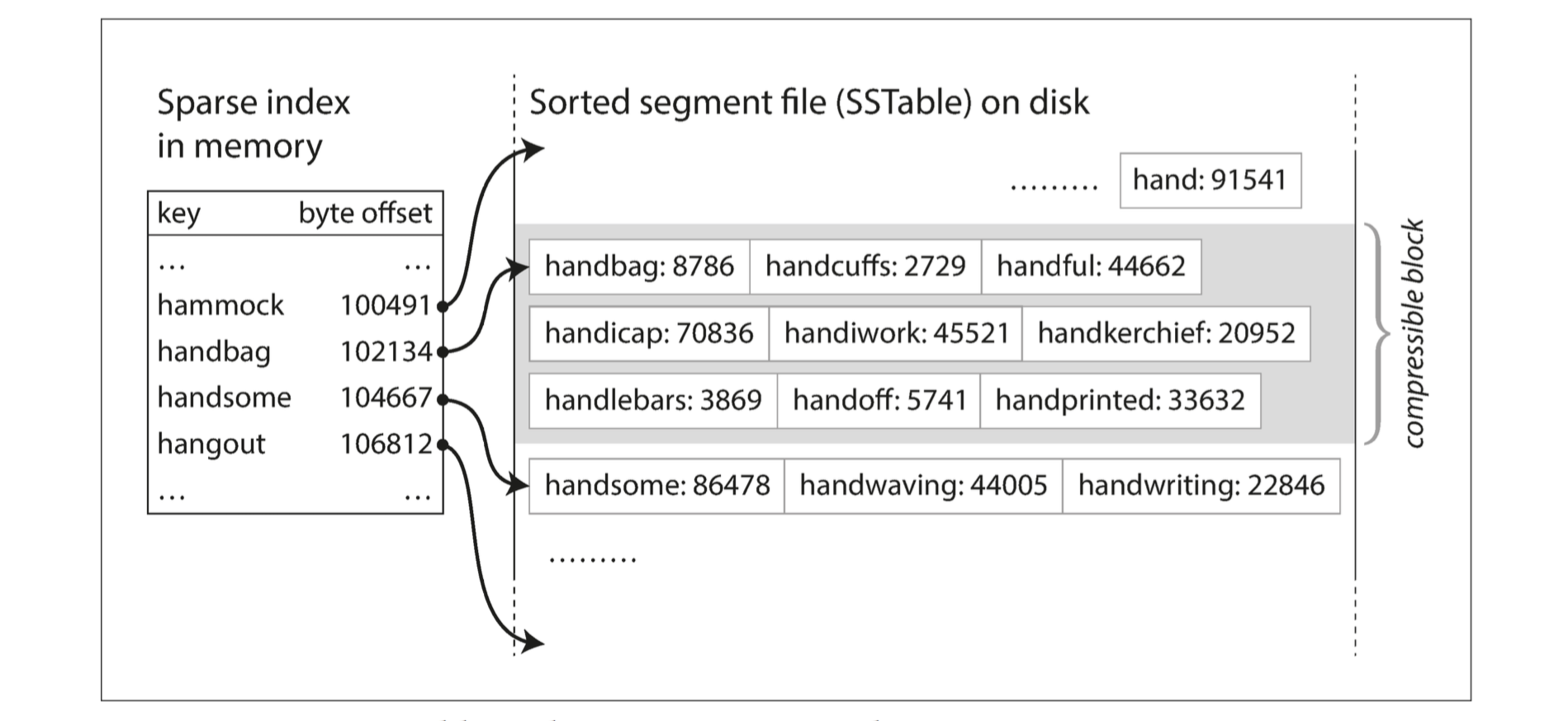
Since read requests need to scan over several key-value pairs in the requested range anyway, it is possible to group those records into a block and compress it before writing it to disk. Each entry of the sparse in-memory index then points at the start of a compressed block. Besides saving disk space, compression also reduces the I/O bandwidth use.

Constructing and maintaining SSTables

How do you get your data to be sorted by key in the first place? We can now make our storage engine work as follows:

When a write comes in, add it to an in-memory balanced tree data structure.
When the memtable gets bigger than some threshold—typically a few megabytes—write it out to disk as an SSTable file.
In order to serve a read request, first try to find the key in the memtable, then in the most recent on-disk segment, then in the next-older segment, etc.
From time to time, run a merging and compaction process in the background to combine segment files and to discard overwritten or deleted values.

It only suffers from one problem: if the database crashes, the most recent writes (which are in the memtable but not yet written out to disk) are lost. In order to avoid that problem, we can keep a separate log on disk to which every write is immediately appended, just like in the previous section. That log is not in sorted order, but that doesn’t matter, because its only purpose is to restore the memtable after a crash.

Performance optimizations

The LSM-tree algorithm can be slow when looking up keys that do not exist in the database: you have to check the memtable, then the segments all the way back to the oldest before you can be sure that the key does not exist. In order to optimize this kind of access, storage engines often use additional Bloom filters.

There are also different strategies to determine the order and timing of how SSTables are compacted and merged. The most common options are size-tiered and leveled compaction.

B-Trees

The most widely used indexing structure is quite different: the B-tree.

Like SSTables, B-trees keep key-value pairs sorted by key, which allows efficient key-value lookups and range queries.

The log-structured indexes we saw earlier break the database down into variable-size segments, typically several megabytes or more in size, and always write a segment sequentially. By contrast, B-trees break the database down into fixed-size blocks or pages, traditionally 4 KB in size (sometimes bigger), and read or write one page at a time.

Each page can be identified using an address or location, which allows one page to refer to another—similar to a pointer, but on disk instead of in memory.

One page is designated as the root of the B-tree; whenever you want to look up a key in the index, you start here. The page contains several keys and references to child pages. Each child is responsible for a continuous range of keys, and the keys between the references indicate where the boundaries between those ranges lie.

The number of references to child pages in one page of the B-tree is called the branching factor. If you want to add a new key, you need to find the page whose range encompasses the new key and add it to that page. If there isn’t enough free space in the page to accommodate the new key, it is split into two half-full pages, and the parent page is updated to account for the new subdivision of key ranges.

This algorithm ensures that the tree remains balanced: a B-tree with n keys always has a depth of O(log n). Most databases can fit into a B-tree that is three or four levels deep, so you don’t need to follow many page references to find the page you are look‐ ing for. (A four-level tree of 4 KB pages with a branching factor of 500 can store up to 256 TB.)

Making B-trees reliable

If you split a page because an insertion caused it to be overfull, you need to write the two pages that were split, and also overwrite their parent page to update the references to the two child pages. This is a dangerous operation, because if the database crashes after only some of the pages have been written, you end up with a corrupted index.

In order to make the database resilient to crashes, it is common for B-tree implementations to include an additional data structure on disk: a write-ahead log (WAL, also known as a redo log). This is an append-only file to which every B-tree modification must be written before it can be applied to the pages of the tree itself. When the database comes back up after a crash, this log is used to restore the B-tree back to a consistent state.

An additional complication of updating pages in place is that careful concurrency control is required if multiple threads are going to access the B-tree at the same time. This is typically done by protecting the tree’s data structures with latches (lightweight locks).

B-tree optimizations

Instead of overwriting pages and maintaining a WAL for crash recovery, some databases (like LMDB) use a copy-on-write scheme. A modified page is written to a different location, and a new version of the parent pages in the tree is created, pointing at the new location.
We can save space in pages by not storing the entire key, but abbreviating it. Especially in pages on the interior of the tree, keys only need to provide enough information to act as boundaries between key ranges. Packing more keys into a page allows the tree to have a higher branching factor, and thus fewer levels.
Additional pointers have been added to the tree. For example, each leaf page may have references to its sibling pages to the left and right, which allows scanning keys in order without jumping back to parent pages.

Comparing B-Trees and LSM-Trees

As a rule of thumb, LSM-trees are typically faster for writes, whereas B-trees are thought to be faster for reads.

Advantages of LSM-trees

A B-tree index must write every piece of data at least twice: once to the write-ahead log, and once to the tree page itself (and perhaps again as pages are split). There is also overhead from having to write an entire page at a time, even if only a few bytes in that page changed.

Log-structured indexes also rewrite data multiple times due to repeated compaction and merging of SSTables.

In write-heavy applications, the performance bottleneck might be the rate at which the database can write to disk.

Moreover, LSM-trees are typically able to sustain higher write throughput than B-trees, partly because they sometimes have lower write amplification, and partly because they sequentially write compact SSTable files rather than having to overwrite several pages in the tree.

Since LSM-trees are not page-oriented and periodically rewrite SSTables to remove fragmentation, they have lower storage overheads, especially when using leveled compaction.

Downsides of LSM-trees

A downside of log-structured storage is that the compaction process can sometimes interfere with the performance of ongoing reads and writes.

An advantage of B-trees is that each key exists in exactly one place in the index, whereas a log-structured storage engine may have multiple copies of the same key in different segments. This aspect makes B-trees attractive in databases that want to offer strong transactional semantics: in many relational databases, transaction isolation is implemented using locks on ranges of keys, and in a B-tree index, those locks can be directly attached to the tree.

Other Indexing Structures

A secondary index can easily be constructed from a key-value index. The main difference is that keys are not unique. This can be solved in two ways: either by making each value in the index a list of matching row identifiers (like a postings list in a full-text index) or by making each key unique by appending a row identifier to it.

Storing values within the index

The key in an index is the thing that queries search for, but the value can be one of two things: it could be the actual row (document, vertex) in question, or it could be a reference to the row stored elsewhere. In the latter case, the place where rows are stored is known as a heap file. The heap file approach is common because it avoids duplicating data when multiple secondary indexes are present: each index just references a location in the heap file, and the actual data is kept in one place.

In some situations, the extra hop from the index to the heap file is too much of a performance penalty for reads, so it can be desirable to store the indexed row directly within an index. This is known as a clustered index. For example, in MySQL’s InnoDB storage engine, the primary key of a table is always a clustered index, and secondary indexes refer to the primary key (rather than a heap file location)（每一个 Secondary Index 包含主健，再根据主键索引找到相应的数据）

Multi-column indexes

The most common type of multi-column index is called a concatenated index, which simply combines several fields into one key by appending one column to another(the index definition specifies in which order the fields are concatenated).

Multi-dimensional indexes are a more general way of querying several columns at once, which is particularly important for geospatial data. One option is to translate a two-dimensional location into a single number using a space-filling curve, and then to use a regular B-tree index. More commonly, specialized spatial indexes such as R-trees are used.

Full-text search and fuzzy indexes

To cope with typos in documents or queries, Lucene is able to search text for words within a certain edit distance.

Lucene uses a SSTable-like structure for its term dictionary. This structure requires a small in-memory index that tells queries at which offset in the sorted file they need to look for a key. In LevelDB, this in-memory index is a sparse collection of some of the keys, but in Lucene, the in-memory index is a finite state automaton over the characters in the keys, similar to a trie. This automaton can be transformed into a Levenshtein automaton, which supports efficient search for words within a given edit distance.

Keeping everything in memory

Counterintuitively, the performance advantage of in-memory databases is not due to the fact that they don’t need to read from disk. Rather, they can be faster because they can avoid the overheads of encoding in-memory data structures in a form that can be written to disk.

Transaction Processing or Analytics?

Data Warehousing

A data warehouse is a separate database that analysts can query to their hearts’ content, without affecting OLTP operations. The data warehouse contains a read-only copy of the data in all the various OLTP systems in the company. Data is extracted from OLTP databases (using either a periodic data dump or a continuous stream of updates), transformed into an analysis-friendly schema, cleaned up, and then loaded into the data warehouse. This process of getting data into the warehouse is known as Extract–Transform–Load (ETL).

A big advantage of using a separate data warehouse, rather than querying OLTP systems directly for analytics, is that the data warehouse can be optimized for analytic access patterns. It turns out that the indexing algorithms discussed in the first half of this chapter work well for OLTP, but are not very good at answering analytic queries.

The divergence between OLTP databases and data warehouses

The data model of a data warehouse is most commonly relational, because SQL is generally a good fit for analytic queries.

Stars and Snowflakes: Schemas for Analytics

A wide range of different data models are used in the realm of transaction processing, depending on the needs of the application. On the other hand, in analytics, there is much less diversity of data models. Many data warehouses are used in a fairly formulaic style, known as a star schema (also known as dimensional modeling).

Column-Oriented Storage

In most OLTP databases, storage is laid out in a row-oriented fashion: all the values from one row of a table are stored next to each other. Document databases are similar: an entire document is typically stored as one contiguous sequence of bytes.

The idea behind column-oriented storage is simple: don’t store all the values from one row together, but store all the values from each column together instead.

Column Compression

Depending on the data in the column, different compression techniques can be used. One technique that is particularly effective in data warehouses is bitmap encoding.

Sort Order in Column Storage

Another advantage of sorted order is that it can help with compression of columns.

Writing to Column-Oriented Storage

Column-oriented storage, compression, and sorting all help to make those read queries faster. However, they have the downside of making writes more difficult.

An update-in-place approach, like B-trees use, is not possible with compressed columns. If you wanted to insert a row in the middle of a sorted table, you would most likely have to rewrite all the column files.

Fortunately, we have already seen a good solution earlier in this chapter: LSM-trees. All writes first go to an in-memory store, where they are added to a sorted structure and prepared for writing to disk. It doesn’t matter whether the in-memory store is row-oriented or column-oriented. When enough writes have accumulated, they are merged with the column files on disk and written to new files in bulk.

Summary

On a high level, we saw that storage engines fall into two broad categories: those optimized for transaction processing (OLTP), and those optimized for analytics (OLAP). There are big differences between the access patterns in those use cases:

OLTP systems are typically user-facing, which means that they may see a huge volume of requests. Disk seek time is often the bottleneck here.
Data warehouses and similar analytic systems are less well known, because they are primarily used by business analysts, not by end users. Disk bandwidth (not seek time) is often the bottleneck here, and column-oriented storage is an increasingly popular solution for this kind of workload.

On the OLTP side, we saw storage engines from two main schools of thought:

The log-structured school, which only permits appending to files and deleting obsolete files, but never updates a file that has been written. Bitcask, SSTables, LSM-trees, LevelDB, Cassandra, HBase, Lucene, and others belong to this group.
The update-in-place school, which treats the disk as a set of fixed-size pages that can be overwritten. B-trees are the biggest example of this philosophy, being used in all major relational databases and also many nonrelational ones.

Analytic workloads are so different from OLTP: when your queries require sequentially scanning across a large number of rows, indexes are much less relevant. Instead it becomes important to encode data very compactly, to minimize the amount of data that the query needs to read from disk.